Randomized Maximum Likelihood Solver

This notebook demonstrates the use of the Randomized Maximum Likelihood Solver (RML) implemented in the Pastas-Plugins package. It compares three groundwater model calibration approaches:

• Least Squares (LS)

• RML with finite-difference (2-point) Jacobian

• RML with empirical Jacobian

The workflow includes generating synthetic observations, defining the Pastas model structure, running calibrations, generating parameter ensembles, and comparing confidence intervals and simulations.

Setup

Packages

The notebook imports numerical and hydrological modeling packages:

import warnings
from typing import Literal

import matplotlib.pyplot as plt
import numpy as np
import pandas as pd
import pastas as ps

from pastas_plugins.pest.solver import RandomizedMaximumLikelihoodSolver

ps.set_log_level("DEBUG")
warnings.filterwarnings("ignore", category=DeprecationWarning)

/home/docs/checkouts/readthedocs.org/user_builds/pastas-plugins/envs/latest/lib/python3.11/site-packages/tqdm/auto.py:21: TqdmWarning: IProgress not found. Please update jupyter and ipywidgets. See https://ipywidgets.readthedocs.io/en/stable/user_install.html

Data

The notebook loads the Wagna dataset and extracts evaporation and precipitation. These serve as input stresses for the RechargeModel.

df = ps.load_dataset("collenteur_2021")["wagna"]
evap = df["evaporation [mm/d]"].rename("evaporation").dropna()
prec = df["precipitation [mm/d]"].rename("precipitation").loc[evap.index]

Helper functions

Some helper functions to quickly setup models and synthetic series

def get_model(obs: pd.Series) -> ps.Model:
    """Creates a standard Pastas model template.

    Adds a RechargeModel with a Gamma response function.

    Parameters
    ----------
    obs : pd.Series
        Observations series for the model.

    Returns
    -------
    ps.Model
        The model with RechargeModel and noise model configured.
    """
    ml = ps.Model(obs, name="synthetic_model")
    sms = []
    rm = ps.RechargeModel(
        prec=prec,
        evap=evap,
        rfunc=ps.Gamma(),
        name="rch",
    )
    sms.append(rm)
    ml.add_stressmodel(sms)
    ml.initialize()
    ml.set_parameter(
        "constant_d",
        pmin=obs.mean() - 4 * obs.std(),
        pmax=obs.mean() + 4 * obs.std(),
    )
    ml.set_parameter(name="rch_a", initial=100.0)

    return ml


def create_synthetic_series(
    noise_std: float = 0.0, freq: Literal["D", "14D"] = "D"
) -> pd.Series:
    """Generates a synthetic groundwater head time series.

    Builds a model with known parameters, simulates the head time series,
    adds Gaussian noise, and resamples to the chosen frequency.

    Parameters
    ----------
    noise_std : float, optional
        Standard deviation of Gaussian noise to add to observations, by default 0.0
    freq : Literal["D", "14D"], optional
        Resampling frequency ("D" for daily, "14D" for 14-day), by default "D"

    Returns
    -------
    pd.Series
        Synthetic groundwater head observations with realistic but controlled values.
    """
    date_range = pd.date_range(tmin, tmax, freq="D")
    obs = pd.Series(0.0, index=date_range, name="head_obs")
    ml = get_model(obs)
    ml.set_parameter("rch_A", initial=rch_A, move_bounds=True)
    ml.set_parameter("rch_n", initial=rch_n, move_bounds=True)
    ml.set_parameter("rch_a", initial=rch_a, move_bounds=True)
    ml.set_parameter("rch_f", initial=rch_f, move_bounds=True)
    ml.set_parameter("constant_d", initial=constant_d, move_bounds=True)
    sim = ml.simulate(tmin=tmin, tmax=tmax)
    if noise_std > 0.0:
        noise = np.random.default_rng(seed=42).normal(0, noise_std, len(sim))
        sim += noise
    sim = ps.timeseries_utils.pandas_equidistant_sample(sim, freq=freq)

    return sim

Constants

A number of synthetic constants (e.g., rch_A, rch_n, etc.) define the “true” parameters used later in the synthetic model generation.

constant_d = 5.0
rch_A = 0.5
rch_n = 1.1
rch_a = 250.0
rch_f = -0.8
tmin = pd.Timestamp("1980-01-01")
tmax = pd.Timestamp("2019-12-31")

noise_std = 0.025

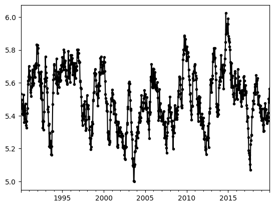
Create a synthetic head series

head = create_synthetic_series(noise_std=noise_std, freq="14D")
head = head.loc[pd.Timestamp("1990-01-01") : tmax]
head.plot(marker=".", color="k")

Model is not optimized yet, initial parameters are used.

<Axes: >

Models

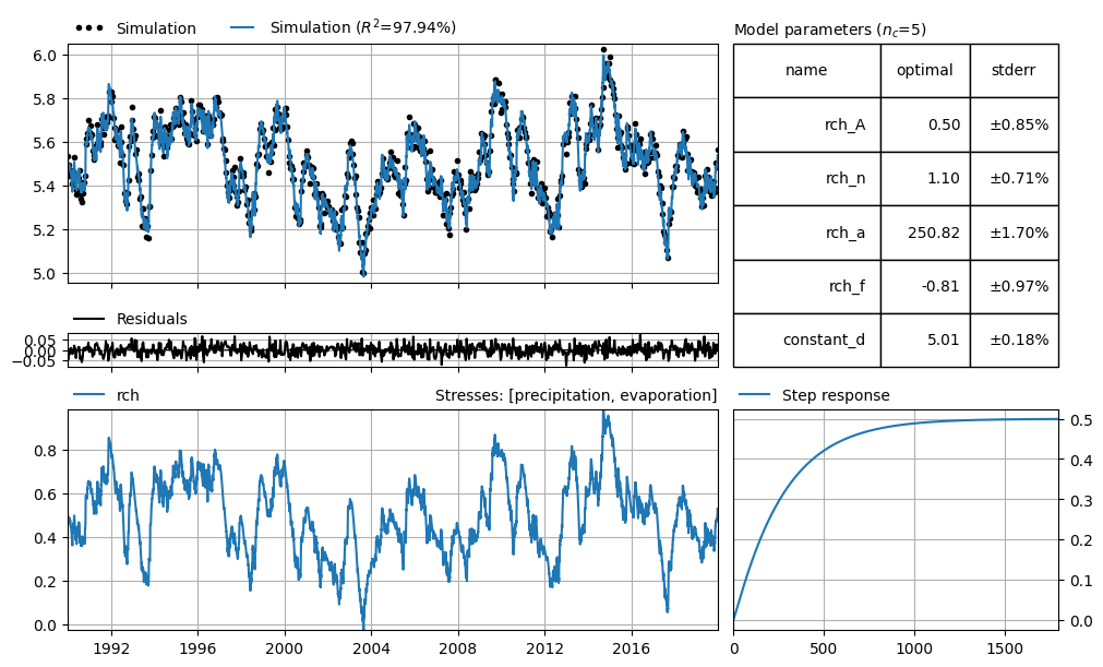
Least Squares

A Pastas model (ml_ls) is calibrated with standard least-squares optimization to show as a baseline model to compare the RML uncertainty estimates.

ml_ls = get_model(head)
ml_ls.solve()
axd = ml_ls.plots.results_mosaic(stderr=True)

DEBUG:pastas.model:[Errno 6] No such device or address

DEBUG:pastas.model:Adding LeastSquares as default solver.

Fit report synthetic_model          Fit Statistics
==================================================
nfev     13                     EVP          97.94
nobs     783                    R2            0.98
noise    False                  RMSE          0.03
tmin     1990-01-02 00:00:00    AICc      -5762.22
tmax     2019-12-24 00:00:00    BIC       -5738.98
freq     D                      Obj           0.25
freq_obs None                   ___               
warmup   3650 days 00:00:00     Interp.         No
solver   LeastSquares           weights        Yes

Parameters (5 optimized)
==================================================
               optimal     initial  vary
rch_A         0.499871    0.146585  True
rch_n         1.098129    1.000000  True
rch_a       250.819346  100.000000  True
rch_f        -0.807632   -1.000000  True
constant_d    5.008214    5.505771  True

RML with finite difference jacobian

In this section we build a model using the Randomized Maximum Likelihood (RML) approach. We apply parameter bounds to constant_d and instantiate the RandomizedMaximumLikelihoodSolver with:

• 250 realizations, forming the RML parameter ensemble

• A three-point finite-difference Jacobian

  • This means each realization performs its own independent optimization starting from its individually drawn initial parameter set.

  • Each realization computes its own finite-difference Jacobian, just like the standard Pastas least-squares solver.

During solver.initialize(), several important steps occur:

• The standard deviation of the observation noise is set via standard_deviation=noise_std. This creates a unique synthetic observation series for each ensemble member, representing uncertainty in the measurement data.

• The arguments method="norm" and par_sigma_range=4.0 define how the initial parameter values for each realization are sampled:

  • method="norm" → initial parameters are drawn from a normal distribution

  • par_sigma_range=4.0 → the parameter bounds (pmin, pmax) are interpreted as ±4 standard deviations of this distribution

Together, these settings define the prior parameter ensemble, from which each realization begins its optimization before contributing to the final RML posterior ensemble.

# test finite difference jacobian
ml_rml = get_model(head)
solver = RandomizedMaximumLikelihoodSolver(
    num_reals=250,
    jacobian_method="2-point",  # other option is 3-point which is slower but more accurate for the jacobian
    # num_workers= # if you want to do stuff in parallel, by default yes. if not set num_workers to 1.
    beta=0.0,  # weighting factor between prior and observation residuals
    minimize_method="SLSQP",  # other options are "trust-constr", "L-BFGS-B" and "TNC"
    noptmax=1000,
)
ml_rml.add_solver(solver)
ml_rml.solver.initialize(
    standard_deviation=noise_std,
    method="norm",
    par_sigma_range=4.0,
)

DEBUG:pastas.model:[Errno 6] No such device or address

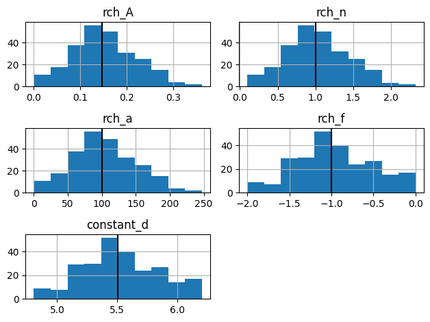
Let’s have a look at the prior parameter ensemble.

axes = ml_rml.solver.parameter_ensemble_prior.hist(bins=10)
for ax in axes.ravel():
    title = ax.get_title()
    if title != "":
        ax.axvline(ml_rml.parameters.at[title, "initial"], color="k", label="initial")
plt.tight_layout()

The observation_noise is stored under the solver.observation_noise:

solver.observation_noise.head()

	0	1	2	3	4	5	6	7	8	9	...	240	241	242	243	244	245	246	247	248	base
1990-01-02	0.006134	0.013955	0.013881	0.004524	0.048632	0.029283	0.071084	0.031424	0.035165	-0.034352	...	0.013375	0.054584	-0.004218	-0.045778	0.059480	0.034920	0.000397	-0.004454	-0.028481	0.0
1990-01-16	-0.014197	-0.008229	0.019937	-0.012047	-0.006529	0.040086	0.015138	0.013051	0.008746	0.020920	...	-0.000361	-0.031685	0.022145	0.014614	0.010912	-0.025800	-0.030544	0.032909	-0.039762	0.0
1990-01-30	0.019058	-0.010101	-0.010682	0.012991	-0.017553	0.002911	-0.000692	0.010395	-0.029478	0.031204	...	-0.001924	-0.030718	-0.003169	0.048684	-0.035050	-0.037988	0.002104	-0.024062	-0.019232	0.0
1990-02-13	0.004715	-0.020735	0.034227	0.020423	-0.029738	0.001357	0.017137	-0.021774	-0.006873	0.013100	...	-0.022094	0.024990	-0.014745	0.008126	0.019464	0.025633	-0.016064	0.014447	0.024804	0.0
1990-02-27	0.036680	0.001687	-0.004078	-0.023111	0.011612	-0.007555	0.001709	-0.031365	0.025758	0.006708	...	0.038635	-0.029654	0.017224	-0.017976	0.029786	0.024733	-0.015048	0.017223	0.009537	0.0

5 rows × 250 columns

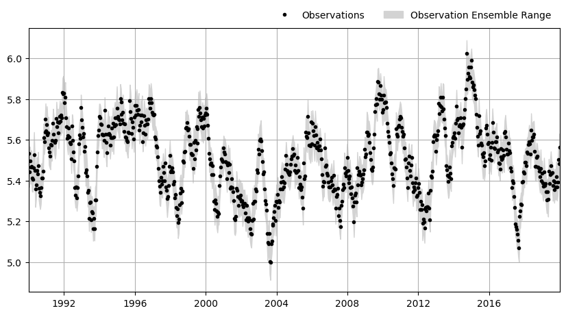
Together with the ml.observations() the observation_noise forms the solver.observation_ensemble on which each ensemble is fitted.

f, ax = plt.subplots(figsize=(10, 5))
ax.plot(
    ml_rml.observations().index,
    ml_rml.observations().values,
    "k.",
    label="Observations",
)
ax.fill_between(
    ml_rml.solver.observation_ensemble.index,
    ml_rml.solver.observation_ensemble.min(axis=1),
    ml_rml.solver.observation_ensemble.max(axis=1),
    color="lightgrey",
    label="Observation Ensemble Range",
)

ax.set_xlim(ml_rml.observations().index.min(), ml_rml.observations().index.max())
ax.grid(True)
ax.legend(loc="lower right", bbox_to_anchor=(1.0, 1.0), ncol=2, frameon=False)

<matplotlib.legend.Legend at 0x73dc0e5cc810>

Let’s solve this. It might take up to a minute if it is done in parallel.

ml_rml.solve(report=True, initalize=False)

ERROR:pastas_plugins.pest.solver:Unexpected keyword arguments: ['initalize'], to solve method. These kwargs will be ignored for now. See issue https://github.com/pastas/pastas/pull/1031.

RML looping over realizations:   0%|          | 0/250 [00:00<?, ?it/s]

RML looping over realizations:   0%|          | 1/250 [00:00<02:10,  1.91it/s]

RML looping over realizations:   1%|          | 2/250 [00:00<01:40,  2.46it/s]

RML looping over realizations:   1%|          | 3/250 [00:01<01:47,  2.30it/s]

RML looping over realizations:   2%|▏         | 4/250 [00:01<01:24,  2.92it/s]

RML looping over realizations:   2%|▏         | 5/250 [00:01<01:20,  3.06it/s]

RML looping over realizations:   2%|▏         | 6/250 [00:02<01:16,  3.21it/s]

RML looping over realizations:   3%|▎         | 7/250 [00:02<01:05,  3.71it/s]

RML looping over realizations:   3%|▎         | 8/250 [00:02<01:17,  3.12it/s]

RML looping over realizations:   4%|▎         | 9/250 [00:03<01:20,  2.98it/s]

RML looping over realizations:   4%|▍         | 10/250 [00:03<01:04,  3.71it/s]

RML looping over realizations:   4%|▍         | 11/250 [00:03<01:21,  2.93it/s]

RML looping over realizations:   5%|▍         | 12/250 [00:03<01:07,  3.55it/s]

RML looping over realizations:   5%|▌         | 13/250 [00:04<01:25,  2.78it/s]

RML looping over realizations:   6%|▌         | 14/250 [00:04<01:13,  3.23it/s]

RML looping over realizations:   6%|▌         | 15/250 [00:05<01:22,  2.85it/s]

RML looping over realizations:   7%|▋         | 17/250 [00:05<01:17,  3.02it/s]

RML looping over realizations:   8%|▊         | 19/250 [00:06<01:08,  3.38it/s]

RML looping over realizations:   8%|▊         | 21/250 [00:06<00:51,  4.41it/s]

RML looping over realizations:   9%|▉         | 22/250 [00:06<00:55,  4.08it/s]

RML looping over realizations:   9%|▉         | 23/250 [00:07<01:00,  3.74it/s]

RML looping over realizations:  10%|▉         | 24/250 [00:07<00:55,  4.05it/s]

RML looping over realizations:  10%|█         | 25/250 [00:07<00:59,  3.79it/s]

RML looping over realizations:  10%|█         | 26/250 [00:07<00:55,  4.07it/s]

RML looping over realizations:  11%|█         | 27/250 [00:08<01:01,  3.60it/s]

RML looping over realizations:  11%|█         | 28/250 [00:08<00:52,  4.25it/s]

RML looping over realizations:  12%|█▏        | 29/250 [00:08<00:56,  3.89it/s]

RML looping over realizations:  12%|█▏        | 30/250 [00:08<00:51,  4.25it/s]

RML looping over realizations:  12%|█▏        | 31/250 [00:09<01:00,  3.64it/s]

RML looping over realizations:  13%|█▎        | 32/250 [00:09<00:51,  4.22it/s]

RML looping over realizations:  13%|█▎        | 33/250 [00:09<00:55,  3.88it/s]

RML looping over realizations:  14%|█▎        | 34/250 [00:09<00:55,  3.90it/s]

RML looping over realizations:  14%|█▍        | 35/250 [00:10<00:54,  3.94it/s]

RML looping over realizations:  14%|█▍        | 36/250 [00:10<00:58,  3.64it/s]

RML looping over realizations:  15%|█▍        | 37/250 [00:10<00:53,  3.98it/s]

RML looping over realizations:  15%|█▌        | 38/250 [00:10<01:00,  3.49it/s]

RML looping over realizations:  16%|█▌        | 39/250 [00:11<00:55,  3.78it/s]

RML looping over realizations:  16%|█▌        | 40/250 [00:11<01:10,  2.99it/s]

RML looping over realizations:  16%|█▋        | 41/250 [00:11<00:59,  3.51it/s]

RML looping over realizations:  17%|█▋        | 42/250 [00:12<01:15,  2.75it/s]

RML looping over realizations:  17%|█▋        | 43/250 [00:12<01:05,  3.14it/s]

RML looping over realizations:  18%|█▊        | 44/250 [00:12<01:00,  3.39it/s]

RML looping over realizations:  18%|█▊        | 45/250 [00:13<01:07,  3.02it/s]

RML looping over realizations:  19%|█▉        | 47/250 [00:13<00:58,  3.49it/s]

RML looping over realizations:  19%|█▉        | 48/250 [00:13<00:52,  3.86it/s]

RML looping over realizations:  20%|█▉        | 49/250 [00:14<01:02,  3.22it/s]

RML looping over realizations:  20%|██        | 51/250 [00:14<01:01,  3.22it/s]

RML looping over realizations:  21%|██        | 53/250 [00:15<00:52,  3.72it/s]

RML looping over realizations:  22%|██▏       | 54/250 [00:15<00:50,  3.90it/s]

RML looping over realizations:  22%|██▏       | 55/250 [00:15<00:57,  3.39it/s]

RML looping over realizations:  23%|██▎       | 57/250 [00:16<00:58,  3.33it/s]

RML looping over realizations:  24%|██▎       | 59/250 [00:17<01:01,  3.12it/s]

RML looping over realizations:  24%|██▍       | 61/250 [00:17<00:43,  4.35it/s]

RML looping over realizations:  25%|██▍       | 62/250 [00:17<00:48,  3.88it/s]

RML looping over realizations:  25%|██▌       | 63/250 [00:17<00:44,  4.18it/s]

RML looping over realizations:  26%|██▌       | 64/250 [00:18<00:54,  3.40it/s]

RML looping over realizations:  26%|██▌       | 65/250 [00:18<00:53,  3.48it/s]

RML looping over realizations:  26%|██▋       | 66/250 [00:18<00:52,  3.53it/s]

RML looping over realizations:  27%|██▋       | 67/250 [00:19<00:57,  3.16it/s]

RML looping over realizations:  27%|██▋       | 68/250 [00:19<00:54,  3.33it/s]

RML looping over realizations:  28%|██▊       | 69/250 [00:19<00:56,  3.20it/s]

RML looping over realizations:  28%|██▊       | 70/250 [00:20<00:56,  3.16it/s]

RML looping over realizations:  28%|██▊       | 71/250 [00:20<00:45,  3.91it/s]

RML looping over realizations:  29%|██▉       | 72/250 [00:20<01:00,  2.95it/s]

RML looping over realizations:  30%|██▉       | 74/250 [00:21<00:52,  3.38it/s]

RML looping over realizations:  30%|███       | 75/250 [00:21<00:43,  4.01it/s]

RML looping over realizations:  30%|███       | 76/250 [00:22<00:57,  3.01it/s]

RML looping over realizations:  31%|███       | 78/250 [00:22<00:52,  3.30it/s]

RML looping over realizations:  32%|███▏      | 79/250 [00:22<00:49,  3.45it/s]

RML looping over realizations:  32%|███▏      | 80/250 [00:23<00:50,  3.38it/s]

RML looping over realizations:  32%|███▏      | 81/250 [00:23<00:42,  3.93it/s]

RML looping over realizations:  33%|███▎      | 82/250 [00:23<00:50,  3.36it/s]

RML looping over realizations:  33%|███▎      | 83/250 [00:24<00:53,  3.13it/s]

RML looping over realizations:  34%|███▎      | 84/250 [00:24<00:43,  3.81it/s]

RML looping over realizations:  34%|███▍      | 85/250 [00:24<00:51,  3.23it/s]

RML looping over realizations:  35%|███▍      | 87/250 [00:24<00:40,  3.99it/s]

RML looping over realizations:  35%|███▌      | 88/250 [00:25<00:35,  4.56it/s]

RML looping over realizations:  36%|███▌      | 89/250 [00:25<00:43,  3.67it/s]

RML looping over realizations:  36%|███▌      | 90/250 [00:25<00:37,  4.31it/s]

RML looping over realizations:  36%|███▋      | 91/250 [00:26<00:50,  3.17it/s]

RML looping over realizations:  37%|███▋      | 93/250 [00:26<00:41,  3.79it/s]

RML looping over realizations:  38%|███▊      | 95/250 [00:27<00:39,  3.90it/s]

RML looping over realizations:  39%|███▉      | 97/250 [00:27<00:40,  3.81it/s]

RML looping over realizations:  40%|███▉      | 99/250 [00:28<00:38,  3.89it/s]

RML looping over realizations:  40%|████      | 101/250 [00:28<00:41,  3.60it/s]

RML looping over realizations:  41%|████      | 103/250 [00:29<00:37,  3.91it/s]

RML looping over realizations:  42%|████▏     | 104/250 [00:29<00:38,  3.84it/s]

RML looping over realizations:  42%|████▏     | 105/250 [00:29<00:38,  3.80it/s]

RML looping over realizations:  42%|████▏     | 105/250 [00:29<00:41,  3.53it/s]

---------------------------------------------------------------------------
KeyboardInterrupt                         Traceback (most recent call last)
Cell In[11], line 1
----> 1 ml_rml.solve(report=True, initalize=False)

File ~/checkouts/readthedocs.org/user_builds/pastas-plugins/envs/latest/lib/python3.11/site-packages/pastas/model.py:1017, in Model.solve(self, tmin, tmax, freq, warmup, noise, solver, report, initial, weights, fit_constant, freq_obs, initialize, **kwargs)
   1014     self.add_solver(solver=solver)
   1016 # Solve model
-> 1017 success, optimal, stderr = self.solver.solve(
   1018     noise=self._settings["noise"], weights=weights, **kwargs
   1019 )
   1020 if not success:
   1021     logger.warning("Model parameters could not be estimated well.")

File ~/checkouts/readthedocs.org/user_builds/pastas-plugins/envs/latest/lib/python3.11/site-packages/pastas_plugins/pest/solver.py:1769, in RandomizedMaximumLikelihoodSolver.solve(self, **kwargs)
   1755 if self.jacobian_method in ("2-point", "3-point"):
   1756     func = partial(
   1757         RandomizedMaximumLikelihoodSolver._least_squares_fd,
   1758         parameter_ensemble=self.parameter_ensemble,
   (...)   1766         noptmax=self.noptmax,
   1767     )
-> 1769     results = process_map(
   1770         func,
   1771         range(self.num_reals),
   1772         max_workers=self.num_workers,
   1773         desc="RML looping over realizations",
   1774         chunksize=1,
   1775     )
   1776     # Concatenate all parameter iterations with proper MultiIndex structure
   1777     parameter_iterations = pd.concat(
   1778         [r.parameter_iterations for r in results],
   1779         keys=[r.real for r in results],
   1780         names=["real", "iteration"],
   1781     )

File ~/checkouts/readthedocs.org/user_builds/pastas-plugins/envs/latest/lib/python3.11/site-packages/tqdm/contrib/concurrent.py:105, in process_map(fn, *iterables, **tqdm_kwargs)
    103     tqdm_kwargs = tqdm_kwargs.copy()
    104     tqdm_kwargs["lock_name"] = "mp_lock"
--> 105 return _executor_map(ProcessPoolExecutor, fn, *iterables, **tqdm_kwargs)

File ~/checkouts/readthedocs.org/user_builds/pastas-plugins/envs/latest/lib/python3.11/site-packages/tqdm/contrib/concurrent.py:51, in _executor_map(PoolExecutor, fn, *iterables, **tqdm_kwargs)
     47 with ensure_lock(tqdm_class, lock_name=lock_name) as lk:
     48     # share lock in case workers are already using `tqdm`
     49     with PoolExecutor(max_workers=max_workers, initializer=tqdm_class.set_lock,
     50                       initargs=(lk,)) as ex:
---> 51         return list(tqdm_class(ex.map(fn, *iterables, chunksize=chunksize), **kwargs))

File ~/checkouts/readthedocs.org/user_builds/pastas-plugins/envs/latest/lib/python3.11/site-packages/tqdm/std.py:1181, in tqdm.__iter__(self)
   1178 time = self._time
   1180 try:
-> 1181     for obj in iterable:
   1182         yield obj
   1183         # Update and possibly print the progressbar.
   1184         # Note: does not call self.update(1) for speed optimisation.

File ~/.asdf/installs/python/3.11.12/lib/python3.11/concurrent/futures/process.py:620, in _chain_from_iterable_of_lists(iterable)
    614 def _chain_from_iterable_of_lists(iterable):
    615     """
    616     Specialized implementation of itertools.chain.from_iterable.
    617     Each item in *iterable* should be a list.  This function is
    618     careful not to keep references to yielded objects.
    619     """
--> 620     for element in iterable:
    621         element.reverse()
    622         while element:

File ~/.asdf/installs/python/3.11.12/lib/python3.11/concurrent/futures/_base.py:619, in Executor.map.<locals>.result_iterator()
    616 while fs:
    617     # Careful not to keep a reference to the popped future
    618     if timeout is None:
--> 619         yield _result_or_cancel(fs.pop())
    620     else:
    621         yield _result_or_cancel(fs.pop(), end_time - time.monotonic())

File ~/.asdf/installs/python/3.11.12/lib/python3.11/concurrent/futures/_base.py:317, in _result_or_cancel(***failed resolving arguments***)
    315 try:
    316     try:
--> 317         return fut.result(timeout)
    318     finally:
    319         fut.cancel()

File ~/.asdf/installs/python/3.11.12/lib/python3.11/concurrent/futures/_base.py:451, in Future.result(self, timeout)
    448 elif self._state == FINISHED:
    449     return self.__get_result()
--> 451 self._condition.wait(timeout)
    453 if self._state in [CANCELLED, CANCELLED_AND_NOTIFIED]:
    454     raise CancelledError()

File ~/.asdf/installs/python/3.11.12/lib/python3.11/threading.py:327, in Condition.wait(self, timeout)
    325 try:    # restore state no matter what (e.g., KeyboardInterrupt)
    326     if timeout is None:
--> 327         waiter.acquire()
    328         gotit = True
    329     else:

KeyboardInterrupt: 

_ = ml_rml.plots.results_mosaic(stderr=True)

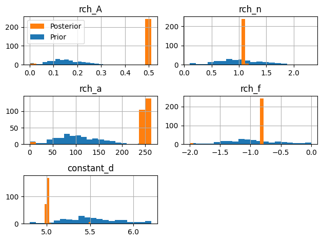
Lets look at the posterior parameter distribution. As you can see the prior is sometimes pretty far away from the posterior. That has to do with how we sample the parameters. Pastas guesses a starting value for pmin, pmax and initial for each parameter (excluding constant_d). If dist= norm then the bounds are sampled as a normal distribution where min(initial-pmin, pmax-initial) is 2 times the standard deviation (par_sigma_range=4.0). This means that if initial is not halfway between pmin and pmax the full extent of the original parameter bounds of Pastas are not sampled. I’m also not sure if I’m fully allowed to call it the posterior.

axes = ml_rml.solver.parameter_ensemble_posterior.hist(bins=20, color="C1")

for i, ax in enumerate(axes.ravel()[:-1]):
    ml_rml.solver.parameter_ensemble_prior.iloc[:, [i]].hist(
        bins=20, ax=ax, zorder=0, color="C0"
    )
axes[0, 0].legend(["Posterior", "Prior"])
plt.tight_layout()

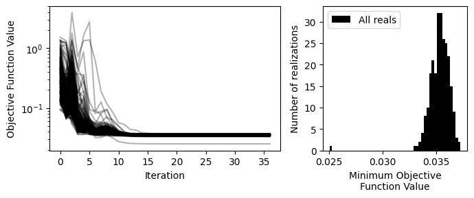
We can also see that some of the posterior values are at bounds or other places. We can have a look at the convergence of realizations and the objective function value.

convergence_rml = ml_rml.solver.convergence_ensemble
print(convergence_rml.value_counts())

converged
True    250
Name: count, dtype: int64

According to SciPy, all realizations converged. If they did not converge (try minimize_method="TNC" for instance), we can get rid of those.

objfuncs_rml = ml_rml.solver.obj_func_ensemble.unstack().loc[convergence_rml].T
min_per_real = (
    ml_rml.solver.obj_func_ensemble.groupby("real").min().loc[convergence_rml]
)
bad_fit_reals = min_per_real[min_per_real > 10.0].index
good_fit_reals = min_per_real[min_per_real <= 10.0].index
f, axd = plt.subplot_mosaic(
    [["iter", "hist"]], figsize=(7.0, 3.0), layout="tight", width_ratios=[1.6, 1]
)
axd["iter"].plot(objfuncs_rml.index, objfuncs_rml.values, "-", color="k", alpha=0.3)
axd["iter"].plot(
    objfuncs_rml.loc[:, bad_fit_reals].index,
    objfuncs_rml.loc[:, bad_fit_reals].values,
    "-",
    color="C1",
    alpha=0.7,
)
axd["iter"].semilogy()
axd["iter"].set_xlabel("Iteration")
axd["iter"].set_ylabel("Objective Function Value")
_, bins, _ = axd["hist"].hist(min_per_real, bins=50, color="k", label="All reals")
axd["hist"].hist(
    min_per_real.loc[bad_fit_reals],
    bins=bins,
    color="C1",
    label="Reals with bad fits",
    alpha=0.5,
)
axd["hist"].set_xlabel("Minimum Objective\nFunction Value")
axd["hist"].set_ylabel("Number of realizations")
axd["hist"].legend()

<matplotlib.legend.Legend at 0x7d7f58838a50>

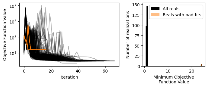
Also looking at the fit of the realizations that did converge; there is a fraction that is in a local minimum. We can get rid of those.

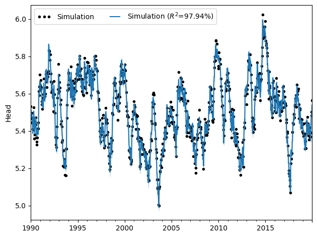
ax = ml_rml.plot()
simulations_rml = ml_rml.solver.simulation_ensemble.loc[:, convergence_rml].loc[
    :, good_fit_reals
]
ax.fill_between(
    simulations_rml.index,
    simulations_rml.quantile(0.025, axis=1),
    simulations_rml.quantile(0.975, axis=1),
    alpha=0.2,
    color="C0",
)

<matplotlib.collections.FillBetweenPolyCollection at 0x7d7f58618050>

Confidence interval is fairly small as is to be expected.

RML with empirical jacobian

There is also an option to try the randomized maximum likelihood solver with the emperical jacobian. Here the jacobian is computed from the parameter ensemble and the simulation ensemble. This method is still a bit experimental because the parameter update is done without lambda searching and lambda is just guessed via lambda = 1e-7 * max(diag(J.T@J)). Also there is no stopping criteria so the number of optimization steps has to be chosen by hand (noptmax).

# test empirical jacobian
ml_rml_em = get_model(head)
solver = RandomizedMaximumLikelihoodSolver(
    num_reals=250,
    jacobian_method="empirical",
    noptmax=100,
    tol=1e-8,
)
ml_rml_em.add_solver(solver)
ml_rml_em.solver.initialize(standard_deviation=noise_std, method="norm")
ml_rml_em.solve(report=True, initialize=False)

DEBUG:pastas.model:[Errno -25] Unknown error -25
RML looping over noptmax:  37%|███▋      | 37/100 [01:21<02:18,  2.19s/it]

Fit report synthetic_model                        Fit Statistics
================================================================
nfev     37                     EVP                        97.94
nobs     783                    R2                          0.98
noise    False                  RMSE                        0.03
tmin     1990-01-02 00:00:00    AICc                    -5762.15
tmax     2019-12-24 00:00:00    BIC                     -5738.91
freq     D                      Obj                         0.03
freq_obs None                   ___                             
warmup   3650 days 00:00:00     Interp.                       No
solver   RandomizedMaximumLikelihoodSolverweights                      Yes

Parameters (5 optimized)
================================================================
               optimal     initial  vary
rch_A         0.500026    0.146585  True
rch_n         1.097864    1.000000  True
rch_a       251.028050  100.000000  True
rch_f        -0.807683   -1.000000  True
constant_d    5.008110    5.505771  True

ml_rml.parameters

	initial	pmin	pmax	vary	name	dist	stderr	optimal
rch_A	0.146585	0.000010	14.658474	True	rch	uniform	0.076473	0.499872
rch_n	1.000000	0.100000	5.000000	True	rch	uniform	0.079312	1.098125
rch_a	100.000000	0.010000	10000.000000	True	rch	uniform	38.796115	250.822144
rch_f	-1.000000	-2.000000	0.000000	True	rch	uniform	0.183148	-0.807632
constant_d	5.505771	4.805792	6.205749	True	constant	uniform	0.077206	5.008213

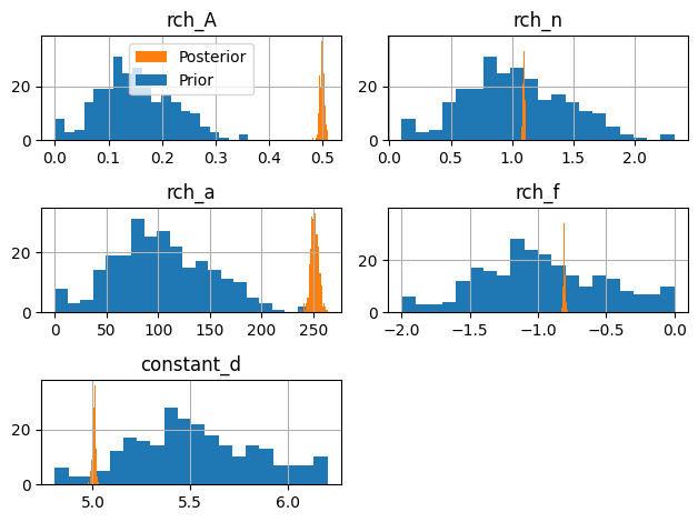
axes = ml_rml_em.solver.parameter_ensemble_posterior.hist(bins=20, color="C1")

for i, ax in enumerate(axes.ravel()[:-1]):
    ml_rml_em.solver.parameter_ensemble_prior.iloc[:, [i]].hist(
        bins=20, ax=ax, zorder=0, color="C0"
    )
axes[0, 0].legend(["Posterior", "Prior"])
plt.tight_layout()

objfuncs_rml_em = ml_rml_em.solver.obj_func_ensemble.unstack().loc[convergence_rml].T
min_per_real_em = (
    ml_rml_em.solver.obj_func_ensemble.groupby("real").min().loc[convergence_rml]
)
f, axd = plt.subplot_mosaic(
    [["iter", "hist"]], figsize=(7.0, 3.0), layout="tight", width_ratios=[1.6, 1]
)
axd["iter"].plot(
    objfuncs_rml_em.index, objfuncs_rml_em.values, "-", color="k", alpha=0.3
)

axd["iter"].semilogy()
axd["iter"].set_xlabel("Iteration")
axd["iter"].set_ylabel("Objective Function Value")
_ = axd["hist"].hist(min_per_real_em, bins=50, color="k", label="All reals")
axd["hist"].set_xlabel("Minimum Objective\nFunction Value")
axd["hist"].set_ylabel("Number of realizations")
axd["hist"].legend()

<matplotlib.legend.Legend at 0x7d7f5b744410>

simulations_rml_em = ml_rml_em.solver.simulation_ensemble
ax = ml_rml_em.plot()
ax.fill_between(
    simulations_rml_em.index,
    simulations_rml_em.quantile(0.025, axis=1),
    simulations_rml_em.quantile(0.975, axis=1),
    alpha=0.2,
    color="C0",
)

<matplotlib.collections.FillBetweenPolyCollection at 0x7d7f584f2fd0>

Compare CI

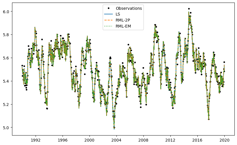
Lets compare the confidence for the different solvers. It can be clearly seen that the confidnece intervalls are fairly similar for the three different solvers. For the emperical jacobian there are some bigger differences that are observed but pretty much negligable.

ls_ci = pd.DataFrame(
    [
        ml_ls.parameters["optimal"] - 1.96 * ml_ls.parameters["stderr"],
        ml_ls.parameters["optimal"],
        ml_ls.parameters["optimal"] + 1.96 * ml_ls.parameters["stderr"],
    ],
    index=[0.025, 0.5, 0.975],
)
rml_ci = (
    ml_rml.solver.parameter_ensemble_posterior.loc[(convergence_rml, slice(None)), :]
    .loc[good_fit_reals]
    .quantile([0.025, 0.5, 0.975])
)
rmlem_ci = ml_rml_em.solver.parameter_ensemble_posterior.quantile([0.025, 0.5, 0.975])
df = pd.concat([ls_ci, rml_ci, rmlem_ci], keys=["LS", "RML-2P", "RML-EM"], axis=1).T
df.swaplevel(0, 1).sort_index().T.round(3)

	constant_d			rch_A			rch_a			rch_f			rch_n
	LS	RML-2P	RML-EM	LS	RML-2P	RML-EM	LS	RML-2P	RML-EM	LS	RML-2P	RML-EM	LS	RML-2P	RML-EM
0.025	4.990	4.989	4.990	0.492	0.492	0.493	242.486	242.457	243.739	-0.823	-0.820	-0.821	1.083	1.081	1.081
0.500	5.008	5.008	5.008	0.500	0.500	0.500	250.819	250.704	250.980	-0.808	-0.807	-0.807	1.098	1.098	1.098
0.975	5.026	5.023	5.023	0.508	0.508	0.508	259.152	259.591	259.420	-0.792	-0.791	-0.791	1.113	1.113	1.112

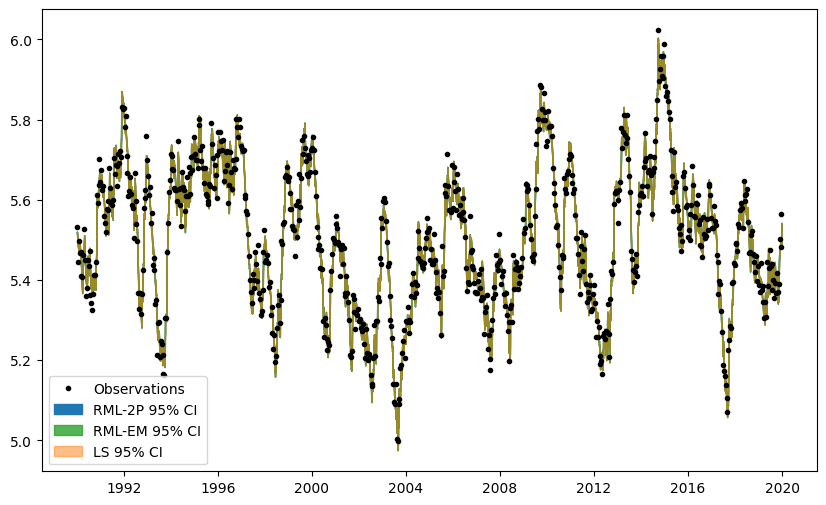
Simulations and confidence intervals in figures also all overlap.

f, ax = plt.subplots(figsize=(10, 6))
ax.plot(
    ml_ls.observations(), label="Observations", color="k", linestyle="None", marker="."
)
ax.plot(ml_ls.simulate(), color="C0", linestyle="-", label="LS")
ax.plot(ml_rml.simulate(), color="C1", linestyle="--", label="RML-2P")
ax.plot(ml_rml_em.simulate(), color="C2", linestyle=":", label="RML-EM")
ax.legend()

<matplotlib.legend.Legend at 0x7d7f584e2990>

f, ax = plt.subplots(figsize=(10, 6))
ax.plot(
    ml_ls.observations(), label="Observations", color="k", linestyle="None", marker="."
)
ax.fill_between(
    simulations_rml.index,
    simulations_rml.quantile(0.025, axis=1),
    simulations_rml.quantile(0.975, axis=1),
    alpha=1.0,
    color="C0",
    label="RML-2P 95% CI",
)
ax.fill_between(
    simulations_rml_em.index,
    simulations_rml_em.quantile(0.025, axis=1),
    simulations_rml_em.quantile(0.975, axis=1),
    alpha=0.8,
    color="C2",
    label="RML-EM 95% CI",
)
ci = ml_ls.solver.ci_simulation(n=100)
ax.fill_between(
    ci.index, ci.iloc[:, 0], ci.iloc[:, 1], color="C1", label="LS 95% CI", alpha=0.5
)
ax.legend()

<matplotlib.legend.Legend at 0x7d7f0d203750>