Using a Modflow DRN model as a stressmodel in Pastas

Please note that the showcased workflow is not how we intend to keep things. Major breaking changes in the next release.

import os

import flopy
import pandas as pd
import pastas as ps

import pastas_plugins.modflow as ppmf

bindir = "bin"
mf6_exe = os.path.join(bindir, "mf6.exe")
if not os.path.isfile(mf6_exe):
    if not os.path.isdir(bindir):
        os.makedirs(bindir)
    flopy.utils.get_modflow("bin", repo="modflow6")

---------------------------------------------------------------------------
ImportError                               Traceback (most recent call last)
Cell In[1], line 7
      4 import pandas as pd
      5 import pastas as ps
----> 7 import pastas_plugins.modflow as ppmf
      9 bindir = "bin"
     10 mf6_exe = os.path.join(bindir, "mf6.exe")

File ~/checkouts/readthedocs.org/user_builds/pastas-plugins/envs/latest/lib/python3.11/site-packages/pastas_plugins/modflow/__init__.py:9
      1 # ruff: noqa: F401
      2 from pastas_plugins.modflow.modflow import (
      3     ModflowDrn,
      4     ModflowDrnSto,
   (...)      7     ModflowUzf,
      8 )
----> 9 from pastas_plugins.modflow.stressmodels import ModflowModel
     10 from pastas_plugins.modflow.version import __version__

File ~/checkouts/readthedocs.org/user_builds/pastas-plugins/envs/latest/lib/python3.11/site-packages/pastas_plugins/modflow/stressmodels.py:7
      5 from pastas.stressmodels import StressModelBase
      6 from pastas.timeseries import TimeSeries
----> 7 from pastas.typing import ArrayLike, TimestampType
      9 from .modflow import Modflow
     11 logger = getLogger(__name__)

ImportError: cannot import name 'TimestampType' from 'pastas.typing' (/home/docs/checkouts/readthedocs.org/user_builds/pastas-plugins/envs/latest/lib/python3.11/site-packages/pastas/typing/__init__.py)

df = pd.read_csv("data/aftopping.csv", index_col=0, parse_dates=True)
head = df["B28H1808_2"].dropna()
prec = df["Precipitation"]
evap = df["Evaporation"]

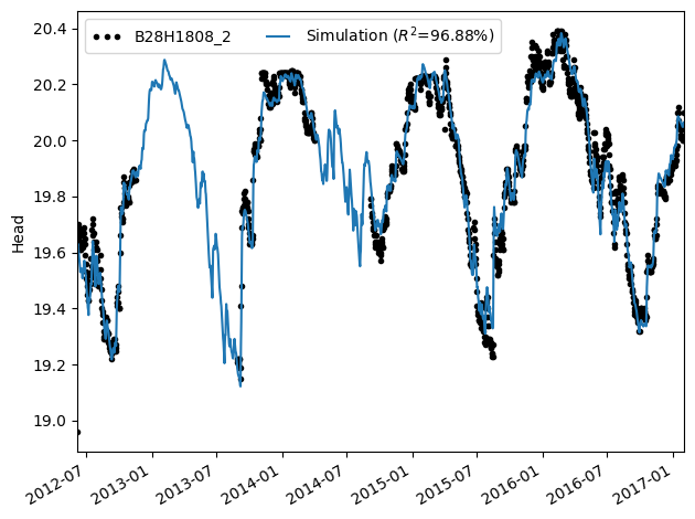
Try to model TARSO with a one cell MODFLOW model

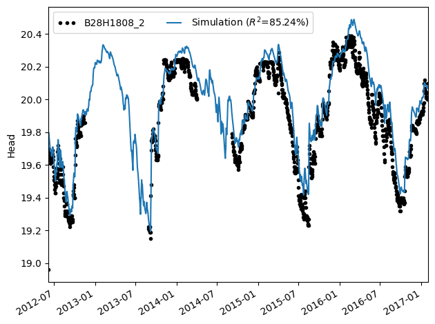
ml_tarso = ps.Model(head, constant=False)
ml_tarso.add_stressmodel(
    ps.TarsoModel(
        prec=prec, evap=evap, rfunc=ps.Exponential(), name="exp", oseries=head
    )
)
ml_tarso.solve()
ml_tarso.plot();

Fit report B28H1808_2             Fit Statistics
================================================
nfev    16                     EVP         96.88
nobs    1261                   R2           0.97
noise   False                  RMSE         0.05
tmin    2012-06-07 00:00:00    AICc     -7360.14
tmax    2017-02-01 00:00:00    BIC      -7324.25
freq    D                      Obj          1.82
warmup  3650 days 00:00:00     ___              
solver  LeastSquares           Interp.        No

Parameters (7 optimized)
================================================
           optimal     initial  vary
exp_A0  661.881263  258.226873  True
exp_a0  117.485675   10.000000  True
exp_d0   19.664685   19.675000  True
exp_A1  368.738780  258.226873  True
exp_a1  138.281724   10.000000  True
exp_d1   20.000696   20.032500  True
exp_f    -1.060276   -1.000000  True

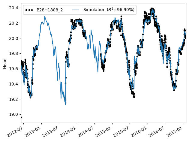
We generate a model with ModflowDrnSto, which adds a drain at a certain threshold-value, and modifies the storage coefficient above this level. If we calculate the parameter-values from the optimized Pastas model with TarsoModel, we see this model returns the same simulation.

# Generate a Model with ModflowDrnSto
ml_mds = ps.Model(head, constant=False)
modflow = ppmf.ModflowDrnSto(
    exe_name=mf6_exe, sim_ws="mf_files/drn_gw", head=head, silent=True
)
mm = ppmf.ModflowModel(prec=prec, evap=evap, modflow=modflow, name="modflow")
ml_mds.add_stressmodel(mm)

# take parameters from the model with the TarsoModel
p_tarso = ml_tarso.parameters["optimal"]
ml_mds.set_parameter(f"{mm.name}_d", initial=p_tarso["exp_d0"])
ml_mds.set_parameter(f"{mm.name}_c", initial=p_tarso["exp_A0"])
s = p_tarso["exp_a0"] / p_tarso["exp_A0"]
ml_mds.set_parameter(f"{mm.name}_s", initial=s)
ml_mds.set_parameter(f"{mm.name}_f", initial=p_tarso["exp_f"])
h_drn = p_tarso["exp_d1"] - p_tarso["exp_d0"]
ml_mds.set_parameter(f"{mm.name}_h_drn", initial=h_drn)
ml_mds.set_parameter(f"{mm.name}_c_drn", initial=p_tarso["exp_A1"])
s_drn = p_tarso["exp_a1"] / p_tarso["exp_A1"]
ml_mds.set_parameter(f"{mm.name}_s_drn", initial=s_drn)

# initialize model and plot
ml_mds.initialize()
ax = ml_mds.plot()

Model is not optimized yet, initial parameters are used.
Model is not optimized yet, initial parameters are used.

ml_mds.parameters

	initial	pmin	pmax	vary	name	dist	stderr	optimal
modflow_d	19.664685	18.960	2.039000e+01	True	modflow	uniform	NaN	NaN
modflow_c	661.881263	10.000	1.000000e+08	True	modflow	uniform	NaN	NaN
modflow_s	0.177503	0.001	5.000000e-01	True	modflow	uniform	NaN	NaN
modflow_f	-1.060276	-2.000	0.000000e+00	True	modflow	uniform	NaN	NaN
modflow_h_drn	0.336012	0.000	1.000000e+01	True	modflow	uniform	NaN	NaN
modflow_c_drn	368.738780	10.000	1.000000e+08	True	modflow	uniform	NaN	NaN
modflow_s_drn	0.375013	0.001	1.000000e+00	True	modflow	uniform	NaN	NaN

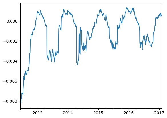
We can plot the difference between the two models. This difference is smaller than the closing criterium of the MODFLOW-model (0.01 meter).

# plot the difference between both models
h1 = ml_tarso.simulate()
h2 = ml_mds.simulate()
(h1 - h2).dropna().plot();

Model is not optimized yet, initial parameters are used.

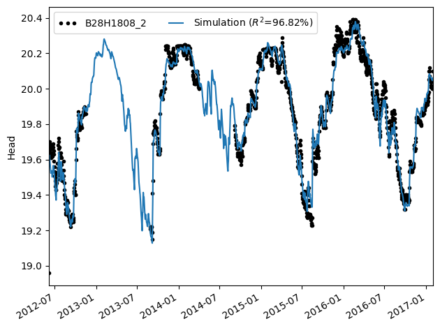
Try to model ThresholdTransform with a one cell MODFLOW model

ml_tt = ps.Model(head)
ml_tt.add_stressmodel(ps.RechargeModel(prec=prec, evap=evap, rfunc=ps.Exponential()))
ml_tt.add_transform(ps.ThresholdTransform())
ml_tt.solve()
ml_tt.plot();

Fit report B28H1808_2               Fit Statistics
==================================================
nfev    26                     EVP           96.82
nobs    1261                   R2             0.97
noise   False                  RMSE           0.05
tmin    2012-06-07 00:00:00    AICc       -7335.76
tmax    2017-02-01 00:00:00    BIC        -7304.99
freq    D                      Obj            1.86
warmup  3650 days 00:00:00     ___                
solver  LeastSquares           Interp.          No

Parameters (6 optimized)
==================================================
                         optimal     initial  vary
recharge_A            594.799905  258.226873  True
recharge_a            103.941136   10.000000  True
recharge_f             -1.060085   -1.000000  True
constant_d             19.658142   19.880246  True
ThresholdTransform_1   20.008782   20.032500  True
ThresholdTransform_2    0.441636    0.500000  True

We try to model this sytyem with ModflowSto. However, this does not give us the same simulation.

ml_ms = ps.Model(head, constant=False)
modflow = ppmf.ModflowSto(
    exe_name=mf6_exe, sim_ws="mf_files/drn_gw", head=head, silent=True
)
mm = ppmf.ModflowModel(prec=prec, evap=evap, modflow=modflow, name="modflow")
ml_ms.add_stressmodel(mm)

p_tt = ml_tt.parameters["optimal"]
ml_ms.set_parameter(f"{mm.name}_d", initial=p_tt["constant_d"])
ml_ms.set_parameter(f"{mm.name}_c", initial=p_tt["recharge_A"])
s = p_tt["recharge_a"] / p_tt["recharge_A"]
ml_ms.set_parameter(f"{mm.name}_s", initial=s)
ml_ms.set_parameter(f"{mm.name}_f", initial=p_tt["recharge_f"])
h_drn = p_tt["ThresholdTransform_1"] - p_tt["constant_d"]
ml_ms.set_parameter(f"{mm.name}_h_drn", initial=h_drn)
s_drn = s / p_tt["ThresholdTransform_2"]
ml_ms.set_parameter(f"{mm.name}_s_drn", initial=s_drn)

ml_ms.initialize()
ax = ml_ms.plot()

Model is not optimized yet, initial parameters are used.
Model is not optimized yet, initial parameters are used.

With ModflowDrnSto we come closer, but we do not get the same result as the Pastas Model with the ThresholdTransform. It is not possible to model the ThresholdTransform in a one-cell Modflow model. ThresholdTransform calculates the discharged water using the non-transformed simulation. However, in the Modflow model, the calculation of the discharge is calculated using the simulation that is affected by the larger storage coefficient.

# Generate a Model with ModflowDrnSto
ml_mds = ps.Model(head, constant=False)
modflow = ppmf.ModflowDrnSto(
    exe_name=mf6_exe, sim_ws="mf_files/drn_gw", head=head, silent=True
)
mm = ppmf.ModflowModel(prec=prec, evap=evap, modflow=modflow, name="modflow")
ml_mds.add_stressmodel(mm)

# take parameters from the model with the TarsoModel
p_tt = ml_tt.parameters["optimal"]
ml_mds.set_parameter(f"{mm.name}_d", initial=p_tt["constant_d"])
ml_mds.set_parameter(f"{mm.name}_c", initial=p_tt["recharge_A"])
s = p_tt["recharge_a"] / p_tt["recharge_A"]
ml_mds.set_parameter(f"{mm.name}_s", initial=s)
ml_mds.set_parameter(f"{mm.name}_f", initial=p_tt["recharge_f"])
h_drn = p_tt["ThresholdTransform_1"] - p_tt["constant_d"]
ml_mds.set_parameter(f"{mm.name}_h_drn", initial=h_drn)
c_drn = p_tt["recharge_A"] * p_tt["ThresholdTransform_2"]
ml_mds.set_parameter(f"{mm.name}_c_drn", initial=c_drn)
s_drn = s / p_tt["ThresholdTransform_2"]
ml_mds.set_parameter(f"{mm.name}_s_drn", initial=s_drn)

# initialize model and plot
ml_mds.initialize()
ax = ml_mds.plot()

Model is not optimized yet, initial parameters are used.
Model is not optimized yet, initial parameters are used.