Benchmark Problem Series J

Benchmark notebook to compare implemented methods to the example from Box et al. (2016).

• Box, G.E.P., Jenkins, G.M., Reinsel G.C., & Greta M. Ljung (2016). Time series analysis: forecasting and control. Fifth edition. John Wiley & Sons, Inc.

Packages

import matplotlib as mpl
import matplotlib.pyplot as plt
import pandas as pd

import pastas_plugins.cross_correlation as ppcc

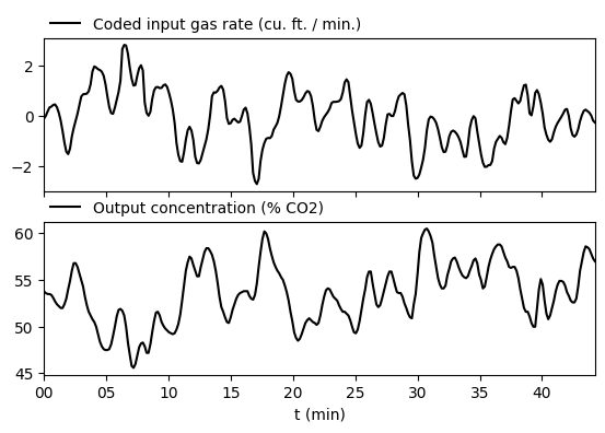
Dataset

seriesj_data = pd.read_csv("data/SeriesJ.csv", index_col=0, parse_dates=True)
X = seriesj_data.loc[:, "Coded input gas rate (cu. ft. / min.)"]
Y = seriesj_data.loc[:, "Output concentration (% CO2)"]

f, ax = plt.subplots(2, 1, sharex=True, figsize=(6.5, 4))
ax[0].plot(X.index, X.values, label=X.name, color="k")
ax[0].legend(loc=(0, 1), frameon=False)
ax[1].plot(Y.index, Y.values, label=Y.name, color="k")
ax[1].legend(loc=(0, 1), frameon=False)
ax[1].set_xlabel("t (min)")
ax[1].xaxis.set_major_locator(mpl.dates.MinuteLocator(interval=5))
ax[1].xaxis.set_major_formatter(mpl.dates.DateFormatter("%M"))
ax[1].set_xlim(X.index[0], X.index[-1]);

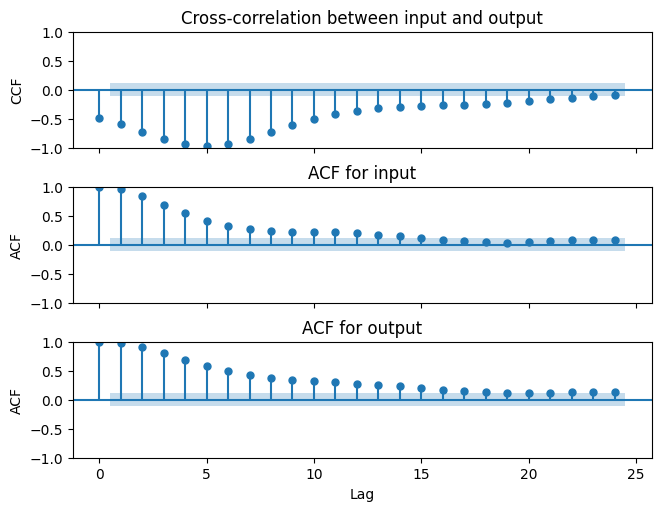
Cross correlation and autocorrelation

nlags = 25
ccf_xy = ppcc.ccf(Y, X, alpha=0.05, nlags=nlags)  # note the order of the arguments
acf_x = ppcc.ccf(X, X, alpha=0.05, nlags=nlags)  # acf is ccf with itself
acf_y = ppcc.ccf(Y, Y, alpha=0.05, nlags=nlags)  # acf is ccf with itself

f, ax = plt.subplots(
    3,
    1,
    sharex=True,
    figsize=(6.5, 5.0),
    constrained_layout=True,
)
ppcc.plot_corr(ccf_xy, ax=ax[0])
ax[0].set_ylabel("CCF")
ax[0].set_title("Cross-correlation between input and output")
ppcc.plot_corr(acf_x, ax=ax[1])
ax[1].set_ylabel("ACF")
ax[1].set_title("ACF for input")
ppcc.plot_corr(acf_y, ax=ax[2])
ax[2].set_ylabel("ACF")
ax[2].set_title("ACF for output")
ax[2].set_xlabel("Lag");

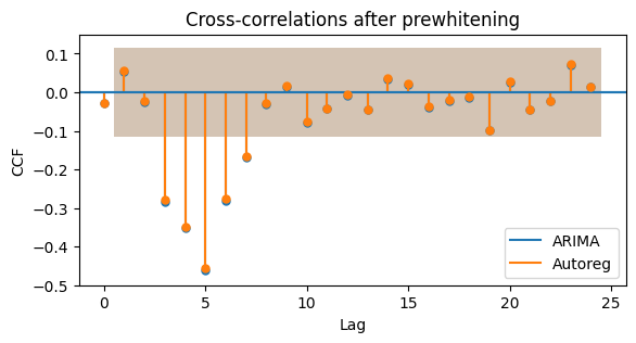
Prewhitening

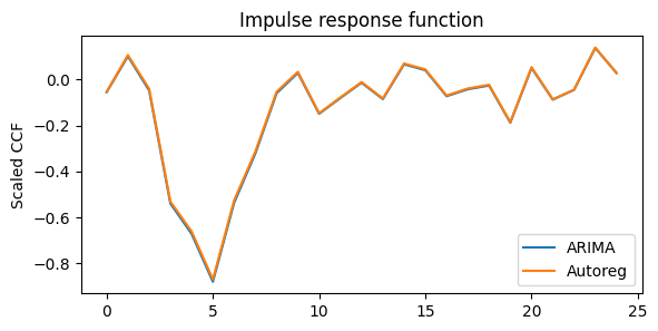
Two options are provided for the autoregressive model that is fitted for prewhitening the input series: ARIMA(p, 0, 0) and AR(p) (Autoreg). The ARIMA model is slightly more accurate but much slower for a large number of lags. The difference with the Autoreg model is very small as is shown below.

p = 4  # order
Xpw_arima, Ypw_arima = ppcc.prewhiten(X, Y, ar=p, arima=True)
Xpw_autoreg, Ypw_autoreg = ppcc.prewhiten(X, Y, ar=p, arima=False)

ccf_arima = ppcc.ccf(Ypw_arima, Xpw_arima, alpha=0.05, nlags=nlags)
ccf_autoreg = ppcc.ccf(Ypw_autoreg, Xpw_autoreg, alpha=0.05, nlags=nlags)

f, ax = plt.subplots(figsize=(6.5, 3.0))
ppcc.plot_corr(ccf_arima, ax, dict(color="C0"))
ppcc.plot_corr(ccf_autoreg, ax, dict(color="C1"))
ax.set_title("Cross-correlations after prewhitening")
ax.set_xlabel("Lag")
ax.set_ylabel("CCF")
ax.plot([], [], color="C0", label="ARIMA")
ax.plot([], [], color="C1", label="Autoreg")
ax.legend()
ax.set_ylim(-0.5, 0.15);

Impulse response function

vk_arima = Ypw_arima.std() / Xpw_arima.std() * ccf_arima.iloc[:, 0]
vk_autoreg = Ypw_autoreg.std() / Xpw_autoreg.std() * ccf_autoreg.iloc[:, 0]

f, ax = plt.subplots(figsize=(6.5, 3.0))
ax.plot(vk_arima.index, vk_arima.values, label="ARIMA")
ax.plot(vk_autoreg.index, vk_autoreg.values, label="Autoreg")
ax.legend()
ax.set_title("Impulse response function")
ax.set_ylabel("Scaled CCF");

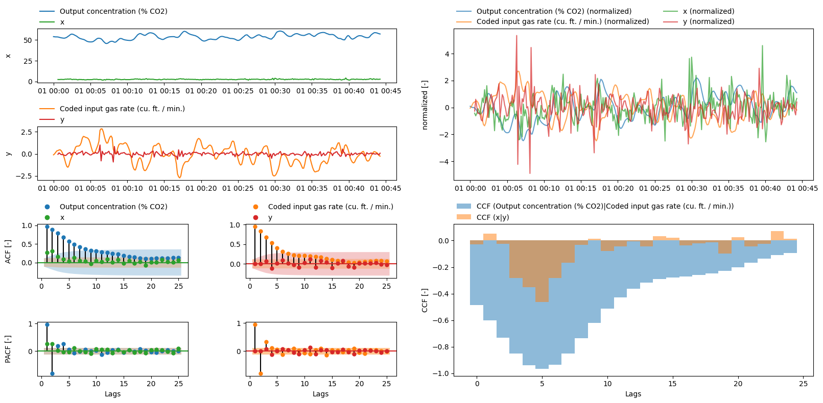
Cross-correlation overview plot

The cross-correlation overview plot allows you to quickly explore the cross-correlation between two time series. The axes can be passed into the function to directly compare the prewhitened result to the original time series.

axes = ppcc.plot_ccf_overview(Y, X, nlags=nlags)
axes = ppcc.plot_ccf_overview(Ypw_arima, Xpw_arima, nlags=nlags, axes=axes)