Using a Modflow model as a stressmodel in Pastas

This notebook shows how to use a simple Modflow model as stress model in Pastas.

Please note that the showcased workflow is not how we intend to keep things. Major breaking changes in the next release.

Packages

import os

import flopy
import pandas as pd
import pastas as ps
from pastas.timer import SolveTimer

import pastas_plugins.modflow as ppmf

ps.set_log_level("ERROR")

/home/docs/checkouts/readthedocs.org/user_builds/pastas-plugins/envs/latest/lib/python3.11/site-packages/tqdm/auto.py:21: TqdmWarning: IProgress not found. Please update jupyter and ipywidgets. See https://ipywidgets.readthedocs.io/en/stable/user_install.html
  from .autonotebook import tqdm as notebook_tqdm

---------------------------------------------------------------------------
ImportError                               Traceback (most recent call last)
Cell In[1], line 8
      5 import pastas as ps
      6 from pastas.timer import SolveTimer
----> 8 import pastas_plugins.modflow as ppmf
     10 ps.set_log_level("ERROR")

File ~/checkouts/readthedocs.org/user_builds/pastas-plugins/envs/latest/lib/python3.11/site-packages/pastas_plugins/modflow/__init__.py:9
      1 # ruff: noqa: F401
      2 from pastas_plugins.modflow.modflow import (
      3     ModflowDrn,
      4     ModflowDrnSto,
   (...)      7     ModflowUzf,
      8 )
----> 9 from pastas_plugins.modflow.stressmodels import ModflowModel
     10 from pastas_plugins.modflow.version import __version__

File ~/checkouts/readthedocs.org/user_builds/pastas-plugins/envs/latest/lib/python3.11/site-packages/pastas_plugins/modflow/stressmodels.py:7
      5 from pastas.stressmodels import StressModelBase
      6 from pastas.timeseries import TimeSeries
----> 7 from pastas.typing import ArrayLike, TimestampType
      9 from .modflow import Modflow
     11 logger = getLogger(__name__)

ImportError: cannot import name 'TimestampType' from 'pastas.typing' (/home/docs/checkouts/readthedocs.org/user_builds/pastas-plugins/envs/latest/lib/python3.11/site-packages/pastas/typing/__init__.py)

Download MODFLOW executable

bindir = "bin"
mf6_exe = os.path.join(bindir, "mf6")
if not os.path.isfile(mf6_exe):
    if not os.path.isdir(bindir):
        os.makedirs(bindir)
    flopy.utils.get_modflow("bin", repo="modflow6")

Data

# %%
tmin = pd.Timestamp("2001-01-01")
tmax = pd.Timestamp("2014-12-31")

tmin_wu = tmin - pd.Timedelta(days=3651)
tmin_wu = pd.Timestamp("1986-01-01")

ds = ps.load_dataset("collenteur_2019")
head = ds["head"].squeeze()
prec = ds["rain"].squeeze().resample("D").asfreq().fillna(0.0)
evap = ds["evap"].squeeze()

# head = pd.read_csv("data/obs.csv", index_col=0, parse_dates=True).squeeze()
# prec = (
#     pd.read_csv("data/rain.csv", index_col=0, parse_dates=True)
#     .squeeze()
#     .resample("D")
#     .asfreq()
#     .fillna(0.0)
# )
# evap = pd.read_csv("data/evap.csv", index_col=0, parse_dates=True).squeeze()

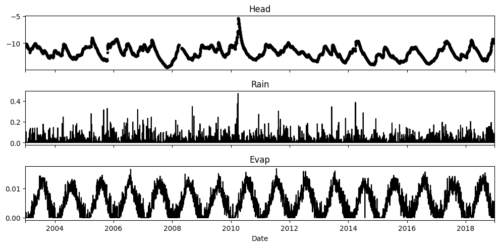
ps.plots.series(head, [prec, evap], hist=False);

Time series models

Standard exponential model

# %%
# create model with exponential response function
mlexp = ps.Model(head)
mlexp.add_stressmodel(
    ps.RechargeModel(prec=prec, evap=evap, rfunc=ps.Exponential(), name="test_exp")
)
mlexp.solve(tmin=tmin, tmax=tmax)
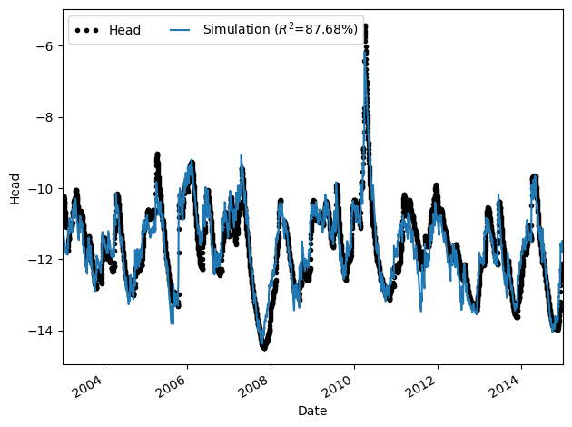
mlexp.plot();

Fit report Head                   Fit Statistics
================================================
nfev    10                     EVP         87.68
nobs    4291                   R2           0.88
noise   False                  RMSE         0.42
tmin    2003-01-01 00:00:00    AICc     -7500.17
tmax    2014-12-31 00:00:00    BIC      -7474.72
freq    D                      Obj        372.93
warmup  3650 days 00:00:00     ___              
solver  LeastSquares           Interp.        No

Parameters (4 optimized)
================================================
               optimal    initial  vary
test_exp_A  341.874957  29.925748  True
test_exp_a   97.909322  10.000000  True
test_exp_f   -0.878938  -1.000000  True
constant_d  -14.227685 -11.740288  True

Uncalibrated MODFLOW time series model

Using parameters based on the Pastas Exponential model.

# %%
# extract resistance and sy from exponential model
# transform exponential parameters to modflow resistance and sy
mlexp_c = mlexp.parameters.loc["test_exp_A", "optimal"]
mlexp_c_i = mlexp.parameters.loc["test_exp_A", "initial"]
mlexp_s = (
    mlexp.parameters.loc["test_exp_a", "optimal"]
    / mlexp.parameters.loc["test_exp_A", "optimal"]
)
mlexp_s_i = (
    mlexp.parameters.loc["test_exp_a", "initial"]
    / mlexp.parameters.loc["test_exp_A", "initial"]
)
mlexp_d = mlexp.parameters.loc["constant_d", "optimal"]
mlexp_d_i = mlexp.parameters.loc["constant_d", "initial"]
mlexp_f = mlexp.parameters.loc["test_exp_f", "optimal"]
mlexp_f_i = mlexp.parameters.loc["test_exp_f", "initial"]

# create modflow pastas model with c and sy
mlexpmf = ps.Model(head)
# shorten the warmup to speed up the modflow calculation somewhat.
mlexpmf.settings["warmup"] = pd.Timedelta(days=4 * 365)
expmf = ppmf.ModflowRch(exe_name=mf6_exe, sim_ws="mf_files/test_expmf", head=head)
expsm = ppmf.ModflowModel(prec=prec, evap=evap, modflow=expmf, name="test_expmfsm")
mlexpmf.add_stressmodel(expsm)
mlexpmf.set_parameter(f"{expsm.name}_s", initial=mlexp_s, vary=False)
mlexpmf.set_parameter(f"{expsm.name}_c", initial=mlexp_c, vary=False)
mlexpmf.set_parameter(f"{expsm.name}_f", initial=mlexp_f, vary=False)
if "constant_d" in mlexpmf.parameters.index:
    mlexpmf.set_parameter("constant_d", initial=mlexp_d, vary=False)
    if expmf._head is not None:
        mlexpmf.del_constant()
        mlexpmf.set_parameter(f"{expsm.name}_d", initial=mlexp_d, vary=False)

sim = mlexpmf.simulate()
ax = mlexpmf.observations().plot(marker=".", color="k", linestyle="None", legend=False)
sim.plot(ax=ax)

<Axes: xlabel='Date'>

mlexpmf.parameters

	initial	pmin	pmax	vary	name	dist	stderr	optimal
test_expmfsm_d	-14.227685	-14.500	-5.420000e+00	False	test_expmfsm	uniform	NaN	NaN
test_expmfsm_c	341.874957	10.000	1.000000e+08	False	test_expmfsm	uniform	NaN	NaN
test_expmfsm_s	0.286389	0.001	5.000000e-01	False	test_expmfsm	uniform	NaN	NaN
test_expmfsm_f	-0.878938	-2.000	0.000000e+00	False	test_expmfsm	uniform	NaN	NaN

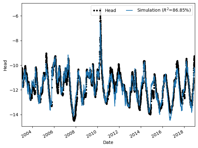
Calibrated MODFLOW time series model

Now fit a Pastas Model using the Modflow model as a response function. This takes some time, as the modflow model has to be recomputed for every iteration in the optimization process.

ml = ps.Model(head)
ml.del_constant()
# shorten the warmup to speed up the modflow calculation somewhat.
ml.settings["warmup"] = pd.Timedelta(days=4 * 365)
mf = ppmf.ModflowRch(exe_name=mf6_exe, sim_ws="mf_files/test_mfrch", head=head)
sm = ppmf.ModflowModel(prec, evap, modflow=mf, name="test_mfsm")
ml.add_stressmodel(sm)

ml.set_parameter(f"{sm.name}_s", initial=mlexp_s_i, vary=True)
ml.set_parameter(f"{sm.name}_c", initial=mlexp_c_i, vary=True)
ml.set_parameter(f"{sm.name}_f", initial=mlexp_f_i, vary=True)
# ml.set_parameter("constant_d", initial=mlexp_d_i, vary=True)

with SolveTimer() as st:
    ml.solve(callback=st.timer)

Optimization progress: 53it [02:19,  2.63s/it]

Fit report Head                   Fit Statistics
================================================
nfev    17                     EVP         86.85
nobs    5737                   R2           0.87
noise   False                  RMSE         0.43
tmin    2003-01-01 00:00:00    AICc     -9760.95
tmax    2018-12-25 00:00:00    BIC      -9734.34
freq    D                      Obj        522.56
warmup  1460 days 00:00:00     ___              
solver  LeastSquares           Interp.        No

Parameters (4 optimized)
================================================
                optimal    initial  vary
test_mfsm_d  -13.843900 -11.740288  True
test_mfsm_c  319.022453  29.925748  True
test_mfsm_s    0.315744   0.334160  True
test_mfsm_f   -0.980087  -1.000000  True

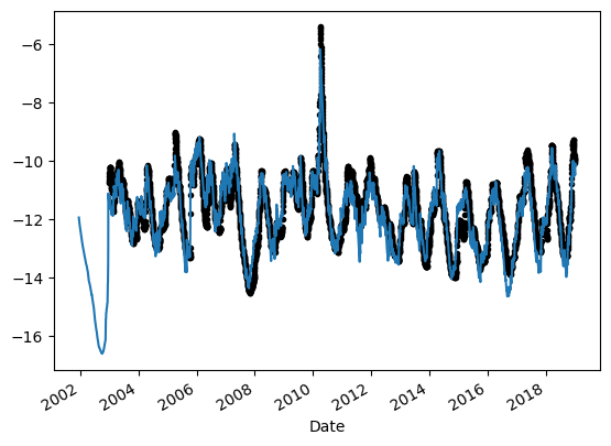
Warnings! (1)
================================================
Response tmax for 'test_mfsm' > than calibration period.

ml.plot();

Results

Parameters

ml.parameters.style.set_table_attributes('style="font-size: 12px"').set_caption(
    "Pastas-Modflow"
)

Pastas-Modflow

	initial	pmin	pmax	vary	name	dist	stderr	optimal
test_mfsm_d	-11.740288	-14.500000	-5.420000	True	test_mfsm	uniform	0.023597	-13.843900
test_mfsm_c	29.925748	10.000000	100000000.000000	True	test_mfsm	uniform	2.552015	319.022453
test_mfsm_s	0.334160	0.001000	0.500000	True	test_mfsm	uniform	0.003336	0.315744
test_mfsm_f	-1.000000	-2.000000	0.000000	True	test_mfsm	uniform	0.004257	-0.980087

mlexp.parameters.style.set_table_attributes('style="font-size: 12px"').set_caption(
    "Pastas-Exponential"
)

Pastas-Exponential

	initial	pmin	pmax	vary	name	dist	stderr	optimal
test_exp_A	29.925748	0.000010	2992.574763	True	test_exp	uniform	2.845206	341.874957
test_exp_a	10.000000	0.010000	1000.000000	True	test_exp	uniform	0.895851	97.909322
test_exp_f	-1.000000	-2.000000	0.000000	True	test_exp	uniform	0.010571	-0.878938
constant_d	-11.740288	nan	nan	True	constant	uniform	0.034303	-14.227685

Compare parameters from the Pastas-Modflow model to the “true” parameters derived from the Pastas exponential model.

comparison = pd.DataFrame(
    {
        "True": mlexpmf.parameters["initial"].values,
        "MF6": ml.parameters["optimal"].values,
    },
    index=ml.parameters.index,
)
comparison["Difference"] = comparison["MF6"] - comparison["True"]
comparison["% Difference"] = (comparison["Difference"] / comparison["True"]) * 100
comparison.style.format(precision=2)

	True	MF6	Difference	% Difference
test_mfsm_d	-14.23	-13.84	0.38	-2.70
test_mfsm_c	341.87	319.02	-22.85	-6.68
test_mfsm_s	0.29	0.32	0.03	10.25
test_mfsm_f	-0.88	-0.98	-0.10	11.51

Plots

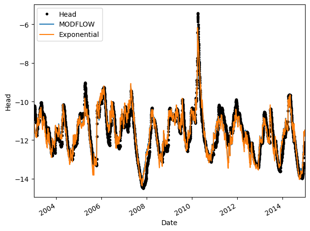
Compare the Pastas-Modflow simulation to the Pastas-Exponential simulation.

ax = ml.plot()  # Pastas-Modflow
mlexp.plot(ax=ax)  # Pastas-Exponential
handles, labels = ax.get_legend_handles_labels()
ax.legend(
    handles[0:2] + handles[3:],
    labels[0:1] + ["MODFLOW", "Exponential"],
    loc="upper left",
)

<matplotlib.legend.Legend at 0x7f63cbf92d40>